Article Goal
My goal is to explain everything you need to know about Markov Decision Processes (MDPs). MDPs are a Markov model or stochastic model used to model randomly changing systems. MDP MDPs are used to describe an environment in reinforcement learning and used for formulating the reinforcement learning problems. They are well suited for reinforcement learning because of the Markov property.
Topics
1. Random Processes and Markov Property
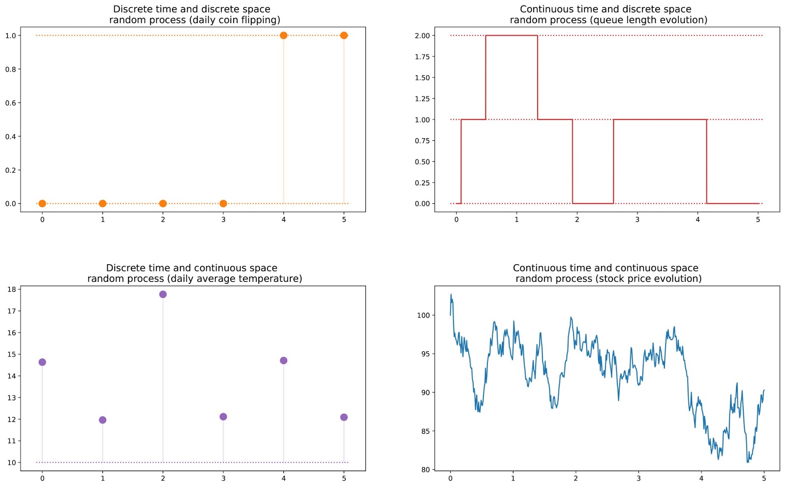
Before we explain Markov processes, we need to learn about random processes (aka stochastic process). Random processes are time-indexed collection of random variables such as the daily price of a stock.
The picture below from here shows different kind of random processes (discrete time vs discrete space, continuous time vs discrete space, discrete time vs continuous space, continuous time vs continuous space).
A random processes can be a Markov Process if it follows the Markov property. Markov property states that the future is independent of the past given its present value. In other words, the markov property expresses the fact that at a given time step and knowing the current state, we won’t get any additional information about the future by gathering information about the past because the current state describes all the past states up until that current state. This is also known as the memoryless property.
To show you an example, consider a ball flying through the air. If the state is position and velocity of the ball, that is sufficient to describe where it has been and where it will go. Therefore, the state has the Markov property. If we only knew the position of the ball but not the velocity, the state is no longer Markov.
Mathematically, the Markov property can written as:
\[P(s_{t+1} | s_{t}, s_{t-1}, s_{t-2}, ...) = P(s_{t+1} | s_{t})\]
2. Types of Markov models
There are four common Markov models used in different situations. Michael Littman’s explanatory grid on Markov Models shows the different situations below.

In reinforcement learning, we will control over the state transitions, and may or may not have states completely observable so we will be concerned mostly with either Markov decision process (MDP) or Partially observable Markov decision process (POMDP) which can be converted to MDPs.
3. Markov Decision Processes (MDPs)
Markov Decision Processes (fully observable environment and control over the state transitions) is a directed graph which has states for nodes and edges which describe transitions between states. All states in MDPs satisfy the Markov property. It is defined by 5-tuple \((S, A, P(s_{t+1}, r \vert s, a), R(s, a, s_{t+1}), \gamma)\):
- \(S\): finite set of possible states.
- \(A\): finite set of possible actions.
- \(P(s_{t+1}, r \vert s, a)\): \(S \times A \rightarrow P\) probability distribution over next state and the reward given current state \(s\), and taking action \(a\).
- \(R(s, a, s_{t+1})\): \(S \times A \rightarrow R\): reward function which gives us a reward for taking action \(a\) in state \(s\) and ending up in \(s_{t+1}\).
- \(\gamma\): discount factor for future rewards which allows us give future rewards less importance than the immediate reward.
The image below shows a MDP. We have:
- Three states \((S_{0}, S_{1}, S_{2})\)
- Two possible action in each state \((a_{0}, a_{1})\)
- Probability transition matrix describing the probability of ending up in a state if action is performed in a state
- Two rewards (\(-1\) from taking \(a_1\) from \(S_2\) and ending up in \(S_0\), \(+5\) from taking \(a_0\) from \(S_1\) and going to \(S_0\))
- \(\gamma\) in this case can be \(1\)
Notice all probabilities of ending up in some state after taking action sum to \(1\).

The goal in reinforcement learning is to learn how to act in a MDP to spend more time in more valuable states so you get high rewards. We can do this by finding an optimal policy \(\bar{\pi}\) which tells us how to act in a particular state to maximize reward. Policies can be stochastic or deterministic.
- Deterministic policies are used in environment where for every state you have a clear defined action you will take.
- Stochastic policies are used in environment where for every state, for you to take an action, you draw a sample from possible actions that follow a distribution.
We will take more about policies in the next article. For now, consider it an oracle which tells you which action is best for you in each state to maximize your reward.
Once we know the optimal policy or a policy, we take actions by following the policy denoted by \(\pi(a \vert s)\). Given a policy \(\pi\), an MDP proceeds as follows:
\[s^{(0)} \rightarrow^{a(0)} s^{(1)} \rightarrow^{a(1)} s^{(2)} \rightarrow^{a(2)} ... \rightarrow^{a(H-1)} s^{H}\]
We take action \(a(0)\) in state \(s(0)\) and end up in state \(s(1)\). We have a reward \(r\) associated with taking action \(a(0)\). When we reach the desired state \(s^H\) or finished taking all the actions, we have completed an episode.
The total accumulated rewards for taking action \(a(0)\) from the first state \(s(0)\) up until taking the last action \(a(H-1)\) to end up in the last state \(s(H)\) is given by:
Total Discounted Reward (TDR) is given by
\(TDR = \gamma^{0} R(s^{(0)}, a^{(0)}, s^{(1)}) + \gamma^{1} R(s^{(1)}, a^{(1)}, s^{(2)}) + \gamma^{2} R(s^{(2)}, a^{(2)}, s^{(3)}) + ... +\gamma^{H-1}R(s^{(H-1)}, a^{(H-1)}, s^{(H)})\)
The discount factor penalizes the rewards in the future because future rewards have higher uncertainty. The \(\gamma\) value is between \([0, 1]\).
Go the next article to learn about how to solve MDPs.